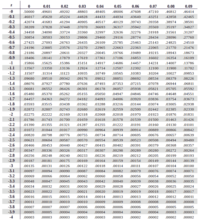
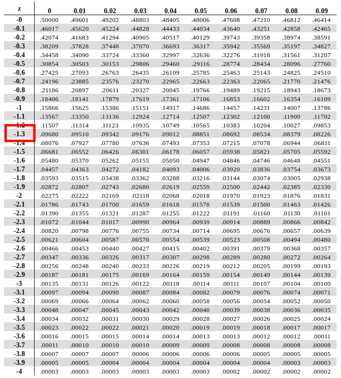
Negative Z score table
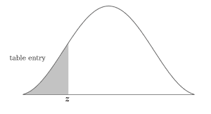
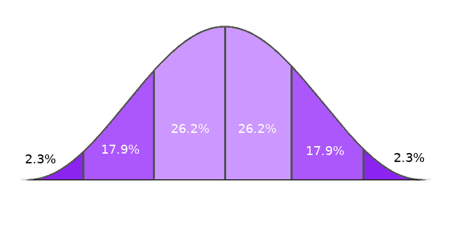
Use the negative Z score table below to find values on the left of the mean as can be seen in the graph alongside. Corresponding values which are less than the mean are marked with a negative score in the z-table and respresent the area under the bell curve to the left of z.
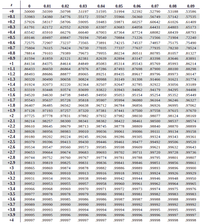
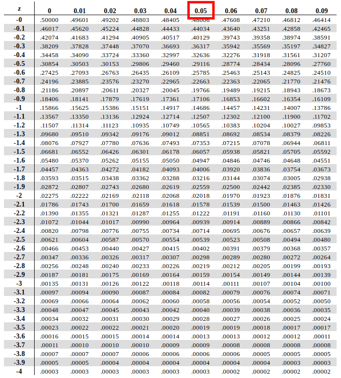
Positive Z score table
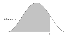
Use the positive Z score table below to find values on the right of the mean as can be seen in the graph alongside. Corresponding values which are greater than the mean are marked with a positive score in the z-table and respresent the area under the bell curve to the left of z.
Note: Feel free to use and share the above images as long as you provide attribution to our site by crediting a link to https://www.ztable.net
How to use the Z Score Formula
To use the Z-Tables however, you will need to know a little something called the Z-Score. It is the Z-Score that gets mapped across the Z-Table and is usually either pre-provided or has to be derived using the Z Score formula. But before we take a look at the formula, let us understand what the Z Score is
What is a Z Score?
A Z Score, also called as the Standard Score, is a measurement of how many standard deviations below or above the population mean a raw score is. Meaning in simple terms, it is Z Score that gives you an idea of a value’s relationship to the mean and how far from the mean a data point is.
A Z Score is measured in terms of standard deviations from the mean. Which means that if Z Score = 1 then that value is one standard deviation from the mean. Whereas if Z Score = 0, it means the value is identical to the mean.
A Z Score can be either positive or negative depending on whether the score lies above the mean (in which case it is positive) or below the mean (in which case it is negative)
Z Score helps us compare results to the normal population or mean
The Z Score Formula
The Z Score Formula or the Standard Score Formula is given as
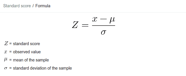
When we do not have a pre-provided Z Score supplied to us, we will use the above formula to calculate the Z Score using the other data available like the observed value, mean of the sample and the standard deviation. Similarly, if we have the standard score provided and are missing any one of the other three values, we can substitute them in the above formula to get the missing value.
Understanding how to use the Z Score Formula with an example
Let us understand how to calculate the Z-score, the Z-Score Formula and use the Z-table with a simple real life example.
Q: 300 college student’s exam scores are tallied at the end of the semester. Eric scored 800 marks (X) in total out of 1000. The average score for the batch was 700 (µ) and the standard deviation was 180 (σ). Let’s find out how well Eric scored compared to his batch mates.
Using the above data we need to first standardize his score and use the respective z-table before we determine how well he performed compared to his batch mates.
To find out the Z score we use the formula
Z Score = (Observed Value – Mean of the Sample)/standard deviation
Z score = ( x – µ ) / σ
Z score = (800-700) / 180
Z score = 0.56
Once we have the Z Score which was derived through the Z Score formula, we can now go to the next part which is understanding how to read the Z Table and map the value of the Z Score we’ve got, using it.
How to Read The Z Table
To map a Z score across a Z Table, it goes without saying that the first thing you need is the Z Score itself. In the above example, we derive that Eric’s Z-score is 0.56.
Once you have the Z Score, the next step is choosing between the two tables. That is choosing between using the negative Z Table and the positive Z Table depending on whether your Z score value is positive or negative.
What we are basically establishing with a positive or negative Z Score is whether your values lie on the left of the mean or right of the mean. To find the area on the left of the mean, you will have a negative Z Score and use a negative Z Table. Similarly, to find the area on the right of the mean, you will have a positive Z Score and use a positive Z Table.
Now that we have Eric’s Z score which we know is a positive 0.56 and we know which corresponding table to pick for it, we will make use of the positive Z-table (Table 1.2) to predict how good or bad Eric performed compared to his batch mates.
Now that we’ve picked the appropriate table to look up to, in the next step of the process we will learn how to map our Z score value in the respective table. Let us understand using the example we’ve chosen with Eric’s Z score of 0.56
Traverse horizontally down the Y-Axis on the leftmost column to find the find the value of the first two digits of your Z Score (0.5 based on Eric’s Z score).
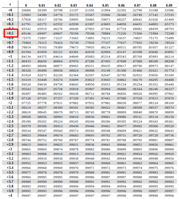
Once you have that, go alongside the X-axis on the topmost row to find the value of the digits at the second decimal position (.06 based on Eric’s Z score)
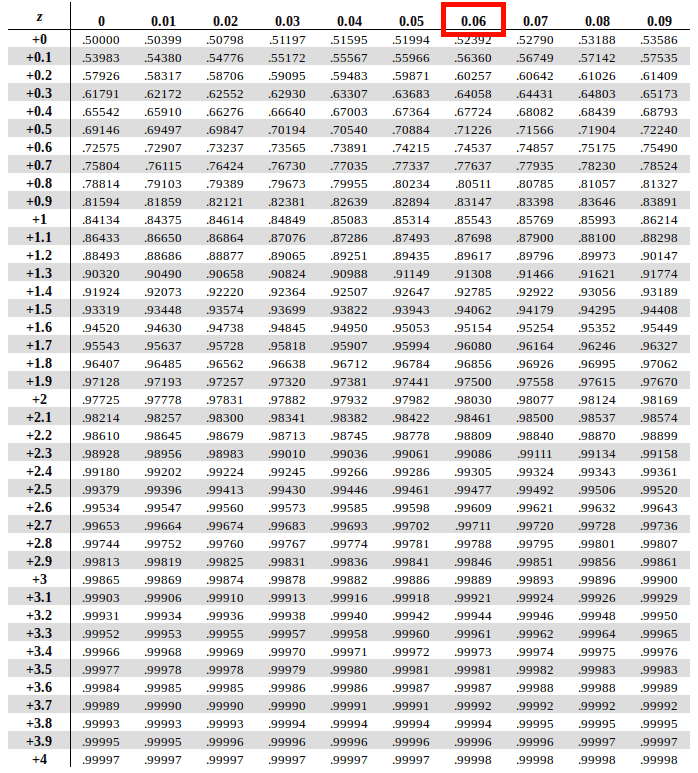
Once you have mapped these two values, find the interesection of the row of the first two digits and column of the second decimal value in the table. The instersection of the two is the answer we’re looking.
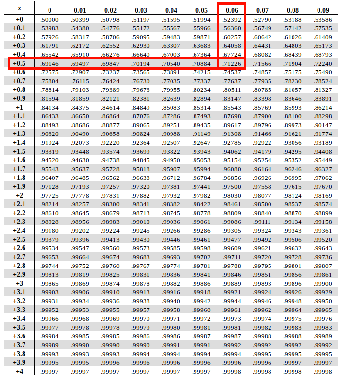
In our example, we get the interesection at a value of 0.71226 (~ 0.7123)
To get this as a percentage we multiply that number with 100. Therefore 0.7123 x 100 = 71.23%. Hence we find out that Eric did better than 71.23% of students.
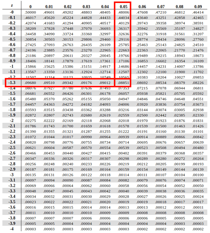
Let us take one more example but this time for a negative z score and a negative z table.
Let us consider our Z score = -1.35
Based on what we had discussed before, since the z score is negative, we will use the negative z table (Table 1.1)
First, traverse horizontally down the Y-Axis on the leftmost column to find the value of the first two digits that is -1.3
Once we have that, we will traverse along the X axis in the topmost row to map the second decimal (0.05 in the case) and find the corresponding column for it.
The interesection of the row of the first two digits and column of the second decimal value in the above Z table is the anwer we’re looking for which in case of our example is 0.08851 or 8.85%
(Note that this method of mapping the Z Score value is same for both the positive as well as the negative Z Scores. That is because for a standard normal distribution table, both halfs of the curves on the either side of the mean are identical. So it only depends on whether the Z Score Value is positive or negative or whether we are looking up the area on the left of the mean or on the right of the mean when it comes to choosing the respective table)
Why are there two Z tables?
There are two Z tables to make things less complicated. Sure it can be combined into one single larger Z-table but that can be a bit overwhelming for a lot of beginners and it also increases the chance of human errors during calculations. Using two Z tables makes life easier such that based on whether you want the know the area from the mean for a positive value or a negative value, you can use the respective Z score table.
If you want to know the area between the mean and a negative value you will use the first table (1.1) shown above which is the left-hand/negative Z-table. If you want to know the area between the mean and a positive value you will the second table (1.2) above which is the right-hand/positive Z-table.
What is Standard Deviation? (σ)
Standard Deviation denoted by the symbol (σ) , the greek letter for sigma, is nothing but the square root of the Variance. Whereas Variance is average of the squared differences from the Mean.
Sample Questions For Practice
1. What is P (Z ≥ 1.20)
Answer: 0.11507
To find out the answer using the above Z-table, we will first look at the corresponding value for the first two digits on the Y axis which is 1.2 and then go to the X axis for find the value for the second decimal which is 0.00. Hence we get the score as 0.11507
2. What is P (Z ≤ 1.20)
(Same as above using the other table. Try solving this yourself for practice)
Answer: 0.88493
History of Standard Normal Distribution Table
The credit for the discovery, origin and penning down the Standard Normal Distribution can be attributed to the 16th century French mathematician Abraham de Moivre ( 26th May 1667 – 27th November 1754) who is well known for his ‘de Moivre’s formula’ which links complex numbers and trigonometry.

De Moivre came about to create the normal distribution through his scientific and math based approach to the gambling. He was trying to come up with a mathematical expression for finding the probabilities of coin flips and various inquisitive aspects of gambling.
He discovered that although data sets can have a wide range of values, we can ‘standardize’ it using a bell shaped distribution curve which makes it easier to analyze data by setting it to a mean of zero and a standard deviation of one. This bell shaped distribution curve that he discovered ended up being known as the normal curve.

This discovery was extremely useful and was put to use by other mathematicians in the years to follow. It was realized that normal distribution applied to a large number of mathematical and real life phenomenas. For example, Belgian astronomer, Lambert Quetelet (22nd February 1796 to 17th February 1874) discovered that despite people’s height, weight and strength presents a big range of dataset with people’s height ranging from 3 to 8 feet and with weight’s ranging from few pounds to few hundred pounds, there was a strong link between people’s height, weight and strength following a standard normal distribution curve.

The normal curve was used not only to standardize the data sets but also to analyze errors and in error distribution patterns. For example, the normal curve was use to analyze errors in astronomical observation measurements. Galileo discovered that the errors were symmetric in nature and in nineteenth century it was realized that even the errors showed a pattern of normal distribution.

The same distribution was also discovered in the late 18th century by the renowned French mathematician Laplace ( Pierre-Simon, marquis de Laplace; 23rd March 1749 to 5th March 1827). Laplace’s central limit theorem states that the distribution of sample means follows the standard normal distribution and that the large the data set the more the distribution deviates towards normal distribution.
Whereas in probability theory a special case of the central limit theorem known as the de Moivre-Laplace theorem states that the normal distribution may be used as an approximation to the binomial distribution under certain conditions. This theorem appears in the second edition pf the book published in 1738 by Abraham de Moivre titled ‘Doctrine of Chances’.
Tags: z table, z score table, normal distribution table, standard normal table, standard normal distribution table, z-table, z-score table, z transform table, ztable,normal table,z value table, z distribution table, z tables, z scores tables, zscore table, z table normal distribution, standard deviation table, z table statistics, z table chart, standard distribution table, z score chart, z-score chart.